Rattle: Data Mining by Example

Welcome to this catalogue of R scripts for data mining. These scripts support and extend the introductory data mining material we find in the Rattle book. We build on the tools provided by Rattle to move from being a novice Rattle data miner into the professional world data mining using R.

The code examples consist of R script files, to be thought of as recipes for particular tasks. These can easily be downloaded and run in R. It probably takes no more than 30 seconds of effort to run each script! Reading this document and also reading the details in the scripts themselves will provide a good introduction of the basics of data mining with R.

I recommend you install RStudio and run the scripts there. We can then step through the scripts one line at a time to learn what is going on. We can also simply run the whole of the script. A nice thing about RStudio is that the sequence of plots generated will be kept in the Plots tab so that we can scroll through them.

See the Data Mining Desktop Survival Guide for much more detail and many more examples.

Some terminology:
observation An entity or object or row of the dataset.
varaible A feature or column of the dataset.

Getting Started

Download (right mouse click on the filename and choose to Save Link As...) the startup and datasets scripts into a folder on your desktop. These are used by most of the other scripts. Then download, for example, dtrees.R into the same folder. Now startup RStudio and under the Tools menu select Set Working Directory and then Browse to that folder. Then Open dtrees.R from the Files tab of the bottom right pane. Run that script within RStudio.

You will notice the use of R environments (as in new.env()) in the examples here. See Chapter 2, page 50 and following, of the Rattle book for an explanation and discussion of why this is a good idea. In short when working with several datasets, several model builders, and in a team of data miners, we can more readily repeat and share the data mining tasks and results as required, by using environments to encapsulate a project. Note that as well as using evalq and with to evaluate expressions within an environment, we ca also, though we don't recommend, attach and detach environments to make their variables available.

Startup

Various functions supporting these examples come from the rattle package. We don't use the Rattle GUI here but we do need to load rattle to access these support functions. The function doRiskChart(), for example, is defined as a shorthand to access the Rattle Risk Chart, as described in Chapter 15 of the Rattle book.

> library("rattle")

Datasets

We use a collection of datasets in these tutorials. These datasets are loaded using this datasets script. The other scripts will generally source() this script to ensure all required datasets are available.

datasets.R The datasets include weatherDS from the rattle package as described in Appendix B of the Rattle book, and irisDS.

Cluster Analysis

Here we demonstrate the kmeans() and our ewkm() algorithms, together with the levelplot.ewkm function which efficiently illustrates the different weights placed on variables relative to each cluster.

kmeans01.R Here we use the traditional kmeans() to construct 10 clusters. The plot provides an indication of how separate the clusters are.

ewkm01.R We use the entropy weighted k-means ewkm() from the siatclust package to generate clusters for the weather dataset. We visualise the relative variable weights (how important each variable is with respect to a cluster). The dendrograms report on the relationship between the clusters and the variables/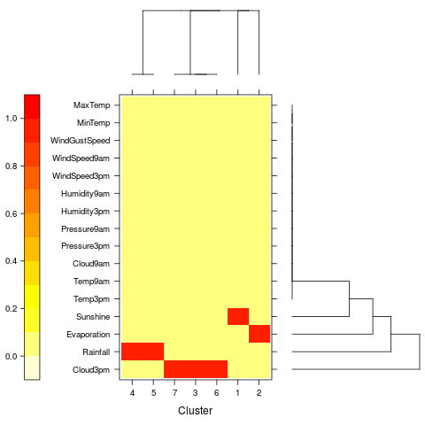

ewkm02.R Again using ewkm() but on the more traditional iris dataset.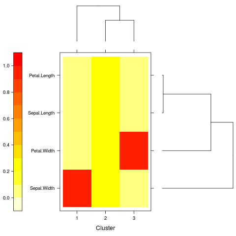

Decision Trees

The common decision tree algorithm is variously implemented by rpart(), ctree(), and CoreModel().

rpart01.R Here we build a traditional decision tree using rpart(). We can read the path through to node 7 as: If the Pressure at 3pm is less than 1011.9 and amount of Sunshine is less than 7.45 hours, then with a 88.9% probability (i.e., very likely) it will rain tomorrow.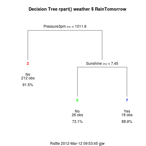

rpart02.R Some prefer a little more gloss in the tree. These trees use prp() from the rpart.plot package. In Rattle we obtain such plots by enabling the Advanced Graphics option in the Settings menu.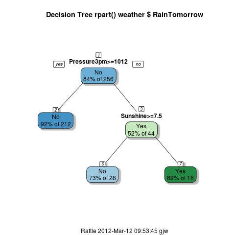

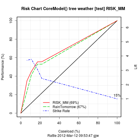
rpart03.R A Risk Chart is a variation of a ROC curve, quite suited to explaining the trade off between a workload (or caseload) on the X axis and the returns on investment (or performance) on the Y axis. They are better explained in a fraud context - to come later.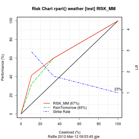

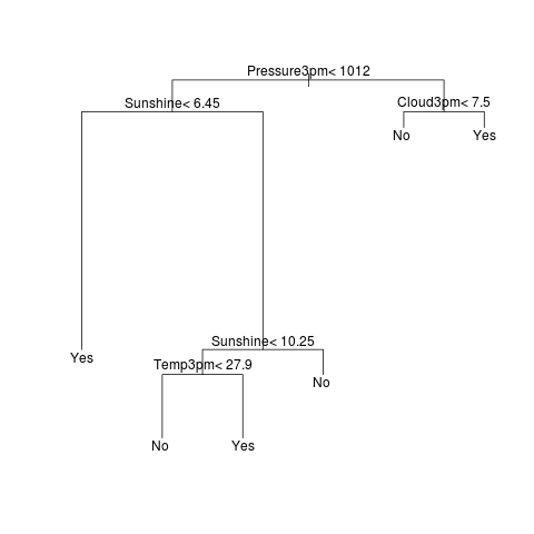
ctree01.R Here we build a conditional decision tree using ctree() from the party package.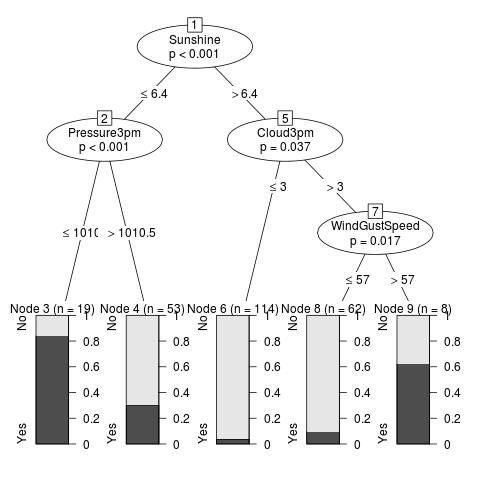

ctree02.R Performance looks better than the rpart() tree.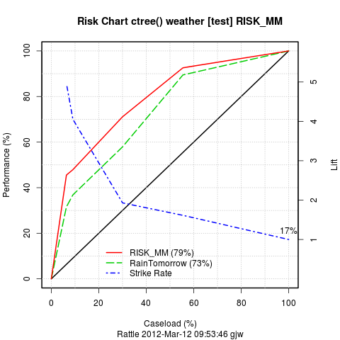

CoreModel01.R

CoreModel02.R

Random Forests

Random forests are my favourite. I started building ensembles of trees in my PhD research in 1987 and have always maintained that they give great results. Here we build forests using randomForest(), cforest(), and CoreModel(model="rf"). Note also the use of predict() to apply the model to new datasets. Click through the Risk Charts to compare the performance of the models. Note how there is randomness involved in building a random forest, thus each time we build a random forest we get different results! We generate 5 plots to show the same randomForest() algorithm on the same data but run at different times (and so with different selections of observations and variables).

rf.R

Have a look at rf_risk_example.pdf for an example of the plot exported from RStudio.

Generlised Linear Model

glm.R

Misc

The following are yet to be tested and have been scouted from various sources.

plots.R

hasse.R

Shop at Amazon